
Making Nice Figures (in MATLAB) - Part 2: EEG timeseries data
Published:
Part Two: EEG timeseries data
This is the second post in a series of posts on making nice figures in MATLAB. In the first post, I introduced some ideas that I think are important for making figures. I definitely leaned on other people’s work, but now I hope to provide some illustrations by building some figures. First, I am going to walk through the process of making an initial figure and cleaning it up to make it publication-ready. I am going to be using electroencephalography (EEG) data throughout the next few posts. The data were recorded during alternating periods of eyes open and eyes closed. This type of data is useful for several reasons. We can start with the timeseries data first and then move on to more complicated representations of the data. The data and code are located here. In addition, you will need the eeglab toolbox. I’ve included everything you need in the repo, but if you plan to continue with EEG data analysis, it is good to stay up to date with the current version of eeglab (also fieldtrip, brainstorm, and many others).
Let’s start by adding eeglab, importing the data, and high-pass filtering it to remove drift. We will select five channels to visualize, not for any specific reason that is relevant to the data, but just to reduce the number of channels to reduce clutter.
clc
clear
close all;

% Add paths
addpath(genpath('utils'));
addpath('eeglab2019_1');
eeglab; clc; clear; close all;

% Load data
load(fullfile(cd,'data','motionTest'));

% Convert to double and transpose. Now data are: [channels x time]
eeg = double(eeg);
eog = double(eog);
fs  = 1000; % Hz

% HP Filter for visualization
eeg = transpose(filterdata('data',eeg,'srate',fs,'highpass',0.3,'highorder',2));
eog = transpose(filterdata('data',eog,'srate',fs,'highpass',0.3,'highorder',2));

% Choose channels to plot: Fp1, Fz, Cz, Pz, Oz
chans2plot = [2, 5, 14, 23, 27];
Version 1
Now lets make our first figure. We are going to visualize the time series using a somewhat brute-force approach. Since they are all approximately zero-mean after filtering, we can just subrtract and offset constant from each one. We will assign each plot to the variable pp so we can clean them up later.
% Define figure window
fig1 = figure('color','w','units','inches','position',[1, 4, 7.5, 5]);

% Get axes
ax = gca;
ax.Box = 'on';

% Define offset for each timeseries
offset = 150;

% Define window to plot
win = eyesOpenIDX(1):eyesOpenIDX(2);

% Initialize empty varaible for each plot
pp = [];

% Plot each EEG timeseries
hold on;
for ii = 1:length(chans2plot)
    % Get channel index
    idx = chans2plot(ii);
    % Offset data
    data = eeg(idx,win) - (ii-1)*offset;
    % Plot data
    pp(ii) = plot(data,'k');

end

%% Make minor adjustments to figure
% Y limits
ylim([-750 200])
% X limits
xlim([0 length(win)])
% Change x and y label
xlabel('Time (sec)')
ylabel('EEG (\muV)')
This is what the produced figure should look like.
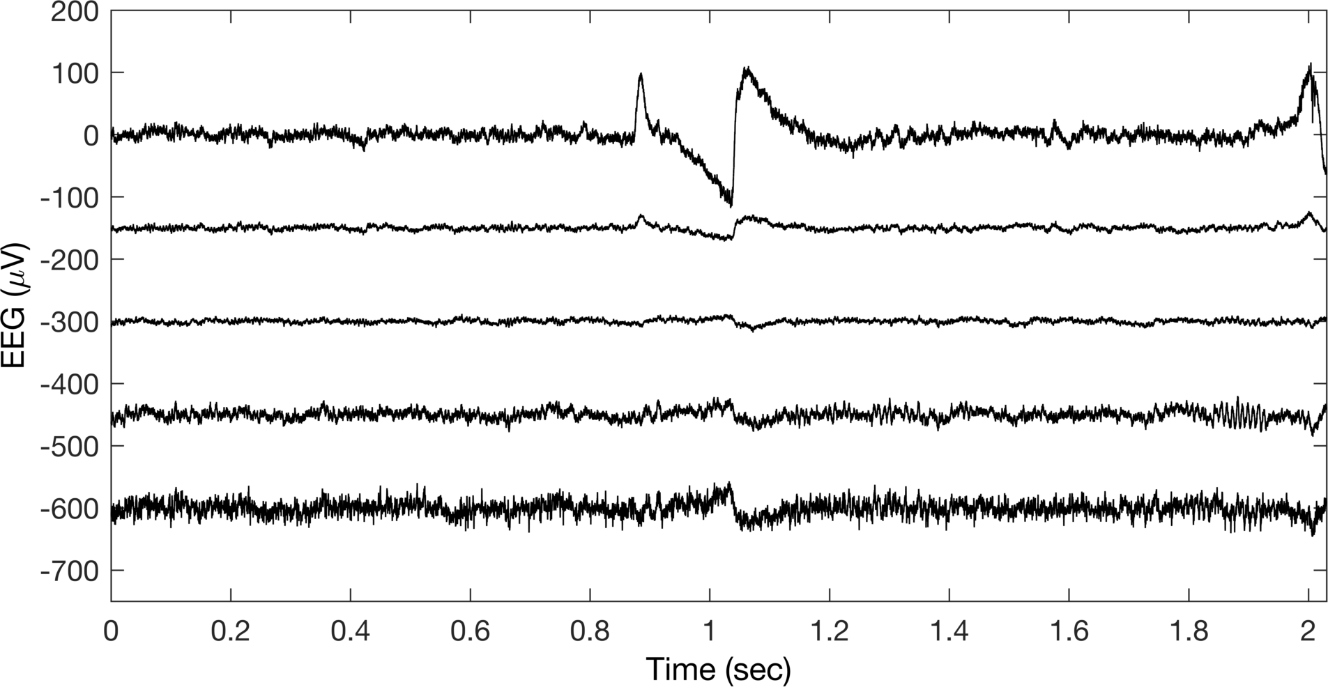
Ok, so this doesn’t look terrible, but I sure would not be happy to put this in a paper or presentation. Let’s try to highlight more about what is happening in the figure. First, let’s label the time when the eyes go from open to closed and change the colors of the channels to differntiate them in a legend.
%% Add line to identify eyes open ---> closed
ll = line([5000 5000],[-750 200],'linestyle','--','color',0.5.*ones(1,3));

%% Change colors of EEG to identify channel names
% Get colorblind colors
colors = blindcolors;
color_ord = [2,3,4,8,6];

% Change each line color
for ii = 1:length(chans2plot)
    all_plot(ii).Color = colors(color_ord(ii),:);
end

% Add legend
leg = legend(all_plot,{'Fp2','Fz','Cz','Pz','Oz'});
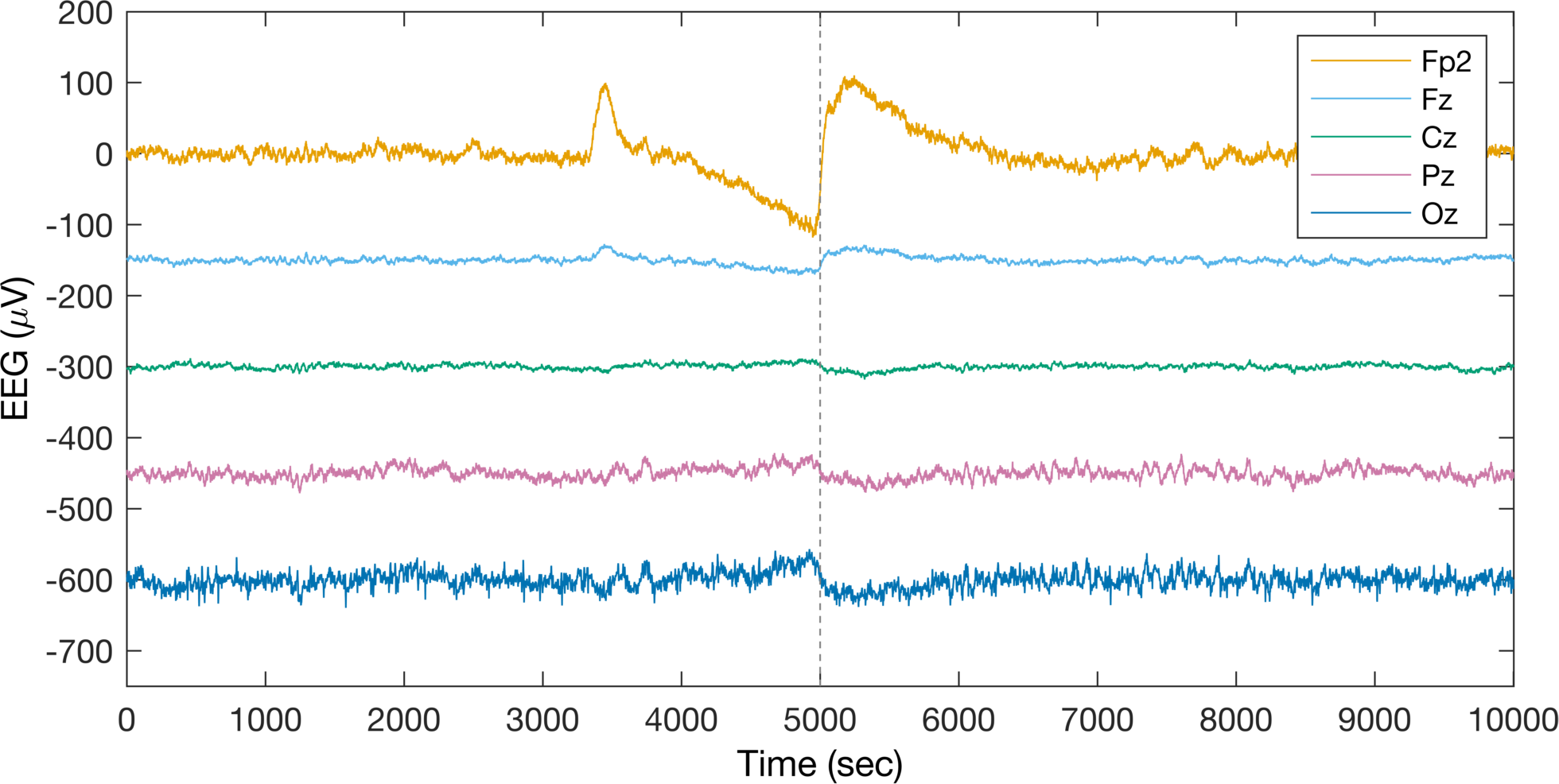
Alright, well this is certainly a way of differentiating individual channels in the legend, but I am not sure I love the way this looks. Let’s instead delete the legend and label the channels by changing their YTickLabel.
%% Changing colors isnt so great - Lets label each of the time series
% Delete the legend
delete(leg);

% Update y ticks based on offset
ax.YTick = fliplr(0 - ((1:length(chans2plot))-1)*150);

% Update y tick labels
ax.YTickLabel = fliplr({'Fp2','Fz','Cz','Pz','Oz'});

% Update x ticks
ax.XTick = (0:10)*fs;
ax.XTickLabel = sprintfc('%d',0:10);

% Add title
title('Eyes Open vs Eyes Closed');

% Change color
for ii = 1:length(chans2plot)
    all_plot(ii).Color = 'k';
end

%% X Ticks should be referenced to event
ax.XTickLabel = sprintfc('%d',-5:5);
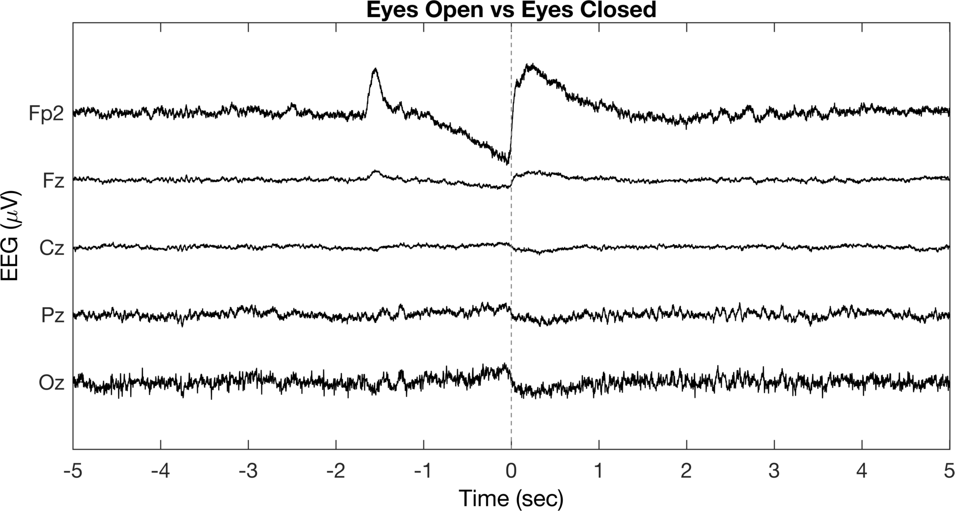
This definitely looks better than the colors and is more informative than the original figure. We’ve labeled the individual channels, identified the time when the eyes switch from open to closed, and referenced the time according to our “event”. However, we can definitely do a lot more to make this better. If you know about EEG data, you might recall that we observe distinct changes in alpha band activity (~8-12 Hz) when eyes are open versus closed. Let’s leverage this information and try to get more out of the figure.
%% Plot alpha data
delete(fig1)
fig1 = figure('color','w','units','inches','position',[1, 4, 7.5, 3.5]);

% Get axes
ax = gca;
ax.Box = 'on';

% Define offset for each timeseries
offset = 15;

% Define window to plot
t = 5;
tt = t*fs;
win = (eyesCloseIDX(1)-tt) : (eyesCloseIDX(1)+tt);

% Initialize empty varaible for each plot
all_plot = [];

% Plot each EEG timeseries
hold on;
for ii = 1:length(chans2plot)
    % Get channel index
    idx = chans2plot(ii);
    % Offset data
    data = eeg_alpha(idx,win) - (ii-1)*offset;
    % Plot data
    pp = plot(data,'k','linewidth',1.1);
    % Add plot to all plot variable
    all_plot = [all_plot; pp];

end

% Y limits
ylim([-offset*length(chans2plot)+offset/2 offset])
% X limits
xlim([0 length(win)])
% Change x and y label
xlabel('Time (sec)')
ylabel('EEG (\muV)')

% Add line to show eyes open vs eyes closed
ll = line([tt tt],ylim,'linestyle','--','color',0.5.*ones(1,3),'linewidth',1.5);

% Update y ticks based on offset
ax.YTick = fliplr(0 - ((1:length(chans2plot))-1)*offset);

% Update y tick labels
ax.YTickLabel = fliplr({'Fp1','Fz','Cz','Pz','Oz'});

% Update x ticks
ax.XTick = (0:2*t)*fs;
ax.XTickLabel = sprintfc('%d',-t:t);

% Add title
title('Eyes Open vs Eyes Closed');
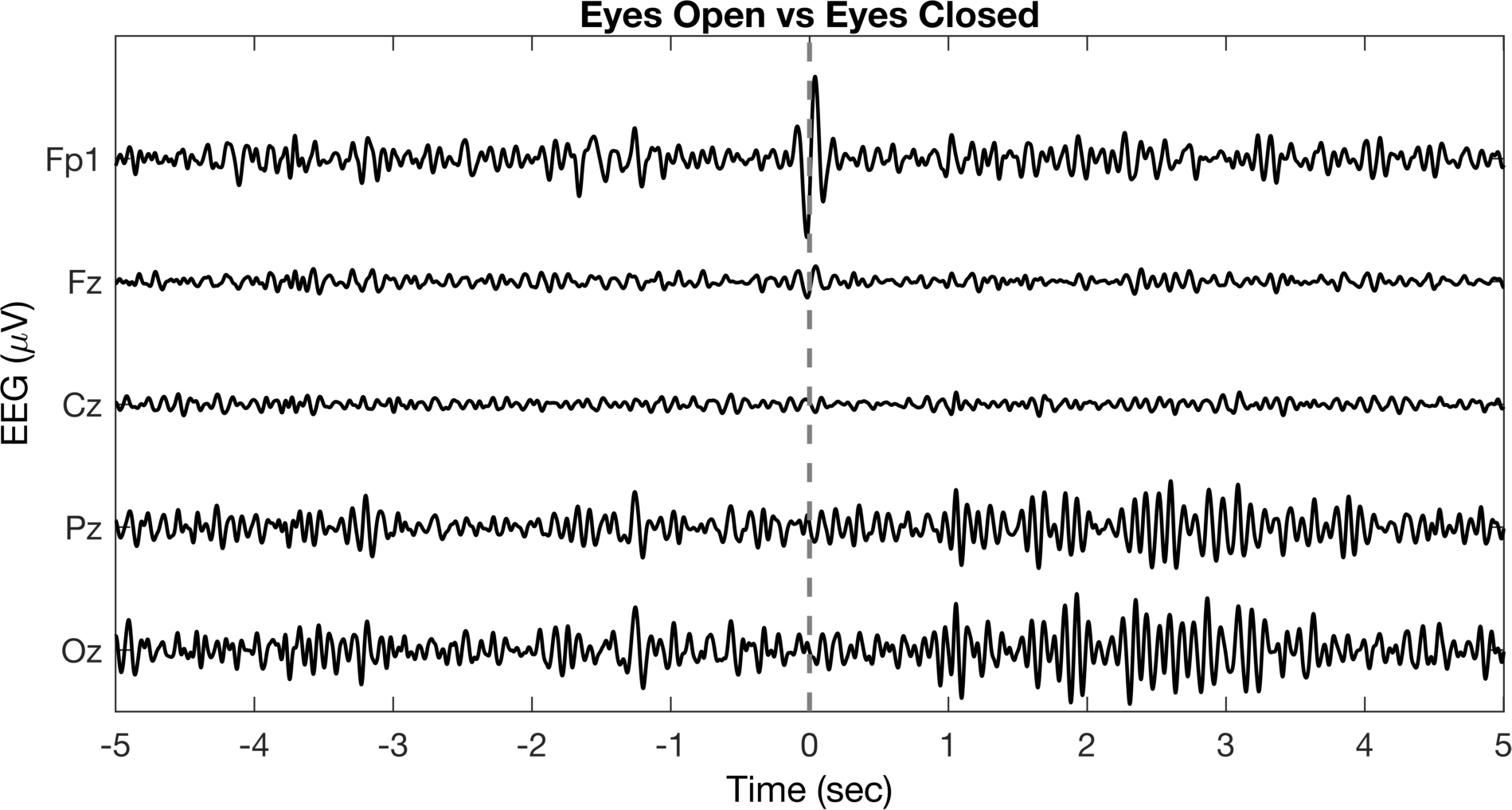
This figure looks much better and has some interesting things going on. We can see the time when we switched from open to closed (filtering does weird things to the blinks, but that’s not a big deal here) and we can see the increased alpha activity in the Pz (parietal) and Oz (occipital) channels along the midline. Again, we can still do more to improve the style and highlight the important aspects of the data.
% Turn off box
ax.Box = 'off';

% Change axis line color to none (can be changed to anything)
ax.XColor = 'none';
ax.YColor = 'none';

% Delete title
ax.Title.String = [];

% Add ax labels back in manually
my_labels = [];
chan_labels = {'Fp2','Fz','Cz','Pz','Oz'};
for ii = 1:length(chans2plot)
    temp = text(-600, -(ii-1)*offset,chan_labels(ii),'fontsize',11,'fontweight','b');
    my_labels = [my_labels; temp];
end

% Add scaling - x axis
xscale = line([0, 1*fs]+100,-offset*length(chans2plot)*ones(1,2)+(offset/2),'color','k','linewidth',1.5);
xscale_text = text(100,-offset*length(chans2plot)+(offset/3),'1 second');

% Add scaling - y axis
xlim([0 length(data)+100])
yscale = line(length(data)+100*ones(1,2), [-5,5] - 2*offset,'color','k','linewidth',1);
yscale_text = text(length(data)+200, - 2*offset, '10 \muV');

% Add labels for eyes open and closed
label_open = text(2000,3*offset/4,'Eyes Open','fontweight','b','fontsize',12);
label_close = text(7000,3*offset/4,'Eyes Closed','fontweight','b','fontsize',12);

%% Highlight certain part of timeseries

% Initialize NaN vectors for each channel
highlight_pz = nan(1,length(data));
highlight_oz = nan(1,length(data));

% Fill in data to plot in different color
highlight_win = 6*fs : 9*fs;
highlight_pz(highlight_win) = all_plot(4).YData(highlight_win);
highlight_oz(highlight_win) = all_plot(5).YData(highlight_win);

% Plot higlight data
p_pz = plot(highlight_pz,'color',colors(8,:),'linewidth',1.1);
p_oz = plot(highlight_oz,'color',colors(6,:),'linewidth',1.1);

% Remove white space to fill figure size
ax.Position = [.075 .05 .85 .9];
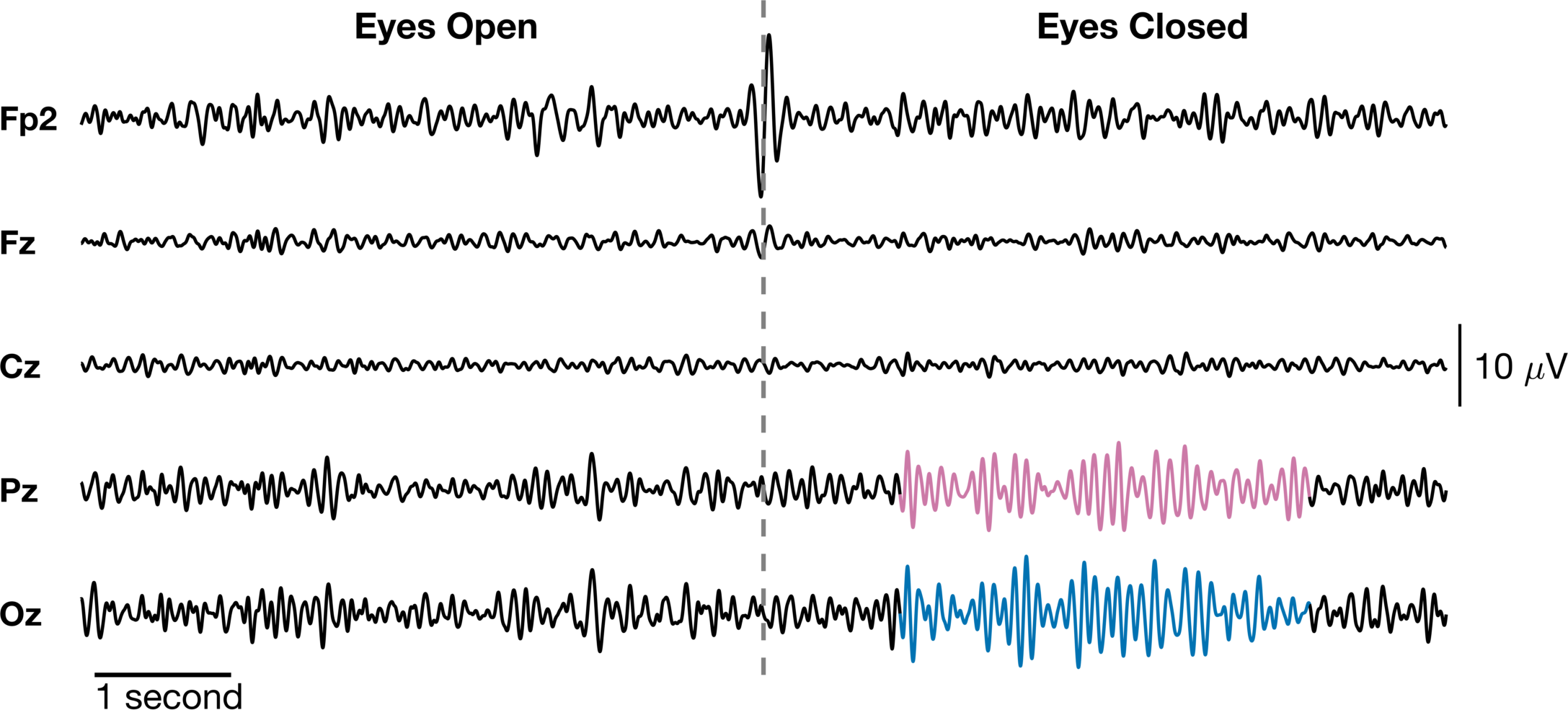
I think this looks great! We have clearly labeled each timeseries and the two distinct events in the data. We labeled the “event onset” and removed the time axis and replaced it with a scale bar for time. Additionally, we highlighted the alpha “bursts” in the Pz and Oz channels and we added scale bars for the amplitude. Just a note, the time scale may not be ideal if you want to reference a specific event and time is important (e.g., N100, P300). Nonetheless, this is a signficantly improved figure from where we started.
Version 2
In the first version, we created a single axis for each time series and offest them using a constant. Although this works, I have observed in the past that it can be problematic when individual timeseries are very different scales. For example, in one of my papers, I needed to create a figure that showed brain, muscle, and joint angle data in the same figure. That would correspond to displaying $\mu V$, $mV$, and degrees using a single constant to scale several orders of magnitude difference and completely different units. In that case, a better approach is to create a single figure window with individual axes for each timeseries. I can still do most of the things I did above, but I have more flexibility and control of each channel.
Let’s start by visualizing a template of what this would look like.
% Define figure
fig2 = figure('color','w','units','inches','position',[1, 4, 7.5, 5]);
% Create axes
% There's a negative value BELOW so that the axes overlap slightly
ax = tight_subplot(5, 1, [-.025 .01] , [.05 .115], [.085 .085]);
for ii = 1:length(ax)
    ax(ii).Box = 'on';
end
% Add axis behind these data axes
ax_pos = [ax(end).Position(1),...
    ax(end).Position(2),...
    ax(end).Position(3),...
    ax(1).Position(2) + ax(1).Position(4)];% - ax(end).Position(2)]; % <-- This would make the top ax_back edge match the top of ax(1)

ax_back = axes('position',ax_pos,'color','r','clipping','off','Box','on');
% Move axis to the bottom
uistack(ax_back,'bottom')
ax_open = axes('color','b','position',[.2, ax(1).Position(2) + ax(1).Position(4) - ax(end).Position(2)/2, .2, .01],'box','on');
ax_closed = axes('color','b','position',[.6, ax(1).Position(2) + ax(1).Position(4) - ax(end).Position(2)/2, .2, .01],'box','on');
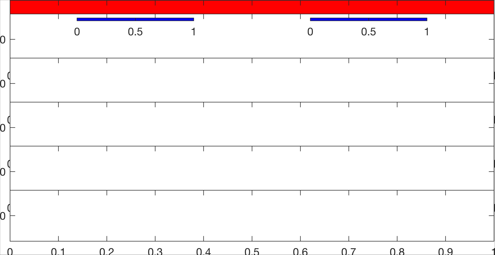
There are several ways to do this, but in my approach, the individual white axes are for each channel. The red is an axis in the back behind the white ones that allows us to label each condition (open vs closed) and create the center line that goes across all channels. The blue one are for some added fun.
fig2 = figure('color','w','units','inches','position',[1, 4, 7.5, 3.5]);
% Create axes - there's a negative value BELOW so that the axes overlap slightly
ax = tight_subplot(5, 1, [-.025 .01] , [.05 .115], [.085 .085]);
% Channel labels
chan_labels = {'Fp2','Fz','Cz','Pz','Oz'};
% Get all data to compute limits
alpha_data = eeg_alpha(chans2plot,win);
minVal = min(alpha_data(:));
maxVal = max(alpha_data(:));
limVal = max(abs([minVal,maxVal]));

% Loop through data and add to each axis
for ii = 1:length(chans2plot)
    % Change which axis is active
    axes(ax(ii));
    % Get channel index
    idx = chans2plot(ii);
    % Offset data
    data = eeg_alpha(idx,win); % No need for offest now: - (ii-1)*offset;
    % Plot data
    pp = plot(data,'k','linewidth',1.1);
    % Change x limits
    ax(ii).XLim = [0 length(win)];

    % Change y limits
    % ax(ii).YLim = [-7.5 7.5];
    ax(ii).YLim = [-limVal limVal];

    % % --------------------------- %
    % % Note: This only works if you dont change the color to 'none'.
    % % Otherwise it also takes the color 'none'.
    % % Add ylabel
    % ax(ii).YLabel.String = chan_labels{ii};
    % % Rotate to 0-deg to make it L/R instead of up/down
    % ax(ii).YLabel.Rotation = 0;
    % % --------------------------- %

    % Turn off axis lines
    ax(ii).XColor = 'none';
    ax(ii).YColor = 'none';

    % Turn off clipping
    ax(ii).Clipping = 'off';
    % Turn off background color so some lines arent cut off
    ax(ii).Color = 'none';

    % Add ax label - add manually using text since we turned off the axis
    % NOTE: the field UserData is empty ([] ) and we can add anything we
    % want to it. Here, we will add a custom y label using text
    ax(ii).UserData.my_ylabel = text(-600, 0, chan_labels(ii),'fontsize',11,'fontweight','b');

end

% Add axis behind these data axes
ax_pos = [ax(end).Position(1),...
    ax(end).Position(2),...
    ax(end).Position(3),...
    ax(1).Position(2) + ax(1).Position(4)];% - ax(end).Position(2)]; % <-- This would make the top ax_back edge match the top of ax(1)

ax_back = axes('position',ax_pos,'color','none','clipping','off');

% Update background axis limits
ax_back.XLim = [0 length(win)];
%ax_back.YLim = [-.15 1];

% Turn off axis lines
ax_back.XColor = 'none';
ax_back.YColor = 'none';

% Move axis to the bottom
% uistack(ax_back,'bottom')

% Add line to show eyes open vs eyes closed
ll = line([tt tt],ylim,'linestyle','--','color',0.5.*ones(1,3),'linewidth',1.5);

% Add scaling - x axis
xscale = line([0, 1*fs]+100,[0 0],'color','k','linewidth',1.5);
xscale_text = text(100,-.03,'1 second');

% Add scaling - y axis
axes(ax(3));
yscale = line(length(data)+100*ones(1,2), [-5,5],'color','k','linewidth',1);
yscale_text = text(length(data)+200, 0, '20 \muV');

% Initialize NaN vectors for each channel
highlight_pz = nan(1,length(data));
highlight_oz = nan(1,length(data));
highlight_win = 6*fs : 9*fs;

% Plot higlight data - Pz
axes(ax(4)); hold on;
highlight_pz(highlight_win) = ax(4).Children(2).YData(highlight_win);
p_pz = plot(highlight_pz,'color',colors(8,:),'linewidth',1.1);

% Plot higlight data - Oz
axes(ax(5)); hold on;
highlight_oz(highlight_win) = ax(5).Children(2).YData(highlight_win);
p_oz = plot(highlight_oz,'color',colors(6,:),'linewidth',1.1);

% Add eyes open/closed labels using titles
ax_open = axes('color','w','position',[.2, ax(1).Position(2) + ax(1).Position(4) - ax(end).Position(2)/2, .2, .01]);
ax_open.Title.String    = 'Eyes Open';
ax_open.Title.FontSize  = 12;
ax_open.XColor = 'none';
ax_open.YColor = 'none';

ax_closed = axes('color','w','position',[.6, ax(1).Position(2) + ax(1).Position(4) - ax(end).Position(2)/2, .2, .01]);
ax_closed.Title.String    = 'Eyes Closed';
ax_closed.Title.FontSize  = 12;
ax_closed.XColor = 'none';
ax_closed.YColor = 'none';
This actually gets us to the same output as the final V1, but we will get a little extra fancy and add some icons.
%% Get fancy and add eye open/closed image
ax_imopen = axes('color','w','position',[.135, ax(1).Position(2) + ax(1).Position(4) - ax(end).Position(2)/2, .1, .1]);
I_open = imread(fullfile('misc','eye_open.png'));
imshow(I_open);

ax_imclosed = axes('color','w','position',[.535, ax(1).Position(2) + ax(1).Position(4) - ax(end).Position(2)/2, .1, .1]);
I_closed = imread(fullfile('misc','eye_closed.png'));
imshow(I_closed);
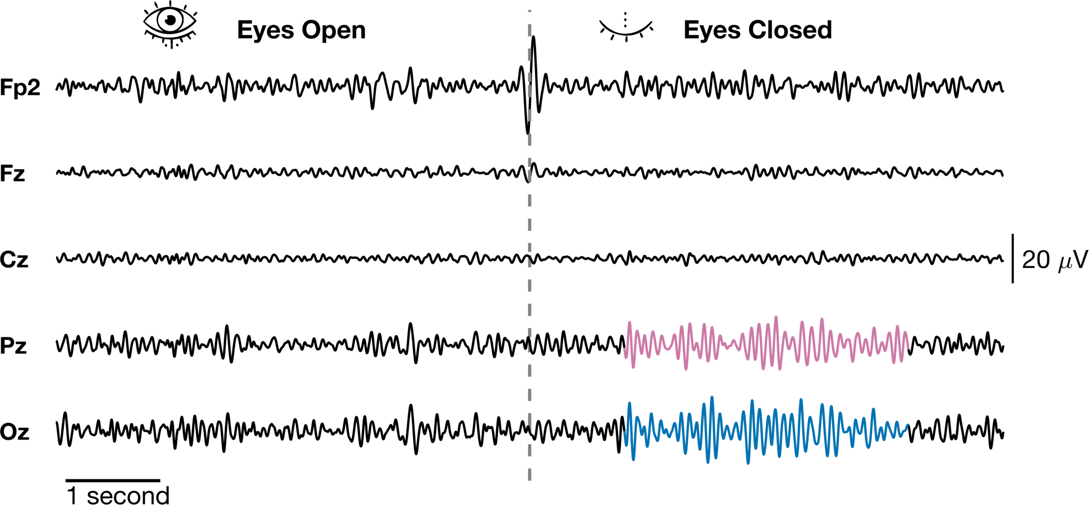
So while this looks pretty much the same as the first one, there are some major differences in the construction. Although these are all on the same scale, we could have accomodated signals of varying amplitude ranges (even orders of magnitude) and simply added scale bars for the different groups. This is what I did in the figure that combined brain, muscle and joint angle data that I referenced before. Here, the scale bars are added to different axes. The time scale bar is added below the Oz axis while the amplitude scale is added to the end of the Cz axis. Another important point is that in order to get the dashed line across all channels, we needed to add an axis on top that spanned all of them. We just set the 'color' = 'none' to make it transparent and set 'xcolor' = 'none' and 'ycolor' = 'none' to turn off the axes completely. Finally, we added to images using the imshow function to their own axes because images do weird things to the axis and it is hard to combine them with other things.
Version 3 - Let’s Animate!
For the final version of this figure, we are going to get super fancy and animate. Again, there are several ways to do this, but I think the best way to do it is by updating your figure for each frame instead of generating a new figure every instance. Basically, we are going to generate an initial figure just like we did before, only this time we will change a few things for the animation.
% Define figure
fig3 = figure('color','w','units','inches','position',[1, 4, 7.5, 3.5]);
% Create axes
% There's a negative value BELOW so that the axes overlap slightly
ax = tight_subplot(5, 1, [-.025 .01] , [.05 .115], [.085 .085]);
% Channel labels
chan_labels = {'Fp2','Fz','Cz','Pz','Oz'};

% Get window of data
alpha_data     = eeg_alpha(chans2plot,eyesOpenIDX(1):eyesOpenIDX(11));
all_alpha_data = eeg_alpha(:,eyesOpenIDX(1):eyesOpenIDX(11));

% Label eyes open/closed
eyes_open = zeros(1,size(alpha_data,2));
events    = [eyesOpenIDX(1:end-1)', eyesCloseIDX(:)] - eyesOpenIDX(1) + 1 ;
for ii = 1:size(events,1)
    eyes_open(events(ii,1):events(ii,2)) = 1;
end

%Compute limits
minVal = min(alpha_data(:));
maxVal = max(alpha_data(:));
limVal = max(abs([minVal,maxVal]));

% Define values for animation
win         = [1 10*fs];
update_rate = 1/25;
win_length  = 1*fs;
stat_win    = [1 win_length];
alpha_power = [];
all_alpha_power = [];

while stat_win(end) < size(alpha_data,2)
    alpha_win = sum(abs(alpha_data(:,stat_win(1):stat_win(2))).^2,2);
    alpha_power = [alpha_power, alpha_win]; % Not efficient!
    all_alpha_power = [all_alpha_power, sum(abs(all_alpha_data(:,stat_win(1):stat_win(2))).^2,2)];;
    stat_win = stat_win + fs*update_rate;
end

% Compute stats on data
mean_alpha = mean(alpha_power(:));
std_alpha  = std(alpha_power(:));
high_power = nan(size(alpha_power));
high_power(alpha_power >= mean_alpha + 3*std_alpha) = 1;

% Mask original data to highlight
alpha_highlight = nan(size(alpha_data));
stat_win    = [1 fs*update_rate];
cnt = 1;
while stat_win(end) < size(alpha_data,2)
    if high_power(cnt) == 1
        alpha_highlight(:,stat_win(1):stat_win(2)) = alpha_data(:,stat_win(1):stat_win(2));
    end
    stat_win = stat_win + fs*update_rate;
    cnt = cnt + 1;
end

% Loop through data and add to each axis
for ii = 1:size(alpha_data,1)
    % Change which axis is active
    axes(ax(ii));

    % Plot data
    pp = plot(alpha_data(ii,win(1):win(2)),'k','linewidth',1.1);
    hold on;
    hl = plot(alpha_highlight(ii,win(1):win(2)),'color',colors(color_ord(ii),:),'linewidth',1.1);

    % Change x limits
    ax(ii).XLim = win;

    % Change y limits
    % ax(ii).YLim = [-7.5 7.5];
    ax(ii).YLim = [-limVal limVal];

    % % --------------------------- %
    % % Note: This only works if you dont change the color to 'none'.
    % % Otherwise it also takes the color 'none'.
    % % Add ylabel
    % ax(ii).YLabel.String = chan_labels{ii};
    % % Rotate to 0-deg to make it L/R instead of up/down
    % ax(ii).YLabel.Rotation = 0;
    % % --------------------------- %

    % Turn off axis lines
    ax(ii).XColor = 'none';
    ax(ii).YColor = 'none';

    % Turn off clipping
    ax(ii).Clipping = 'off';
    % Turn off background color so some lines arent cut off
    ax(ii).Color = 'none';

    % Add ax label - add manually using text since we turned off the axis
    % NOTE: the field UserData is empty ([] ) and we can add anything we
    % want to it. Here, we will add a custom y label using text
    ax(ii).UserData.my_ylabel = text(-600, 0, chan_labels(ii),'fontsize',11,'fontweight','b');

end

% Add axis behind these data axes
ax_pos = [ax(end).Position(1),...
    ax(end).Position(2),...
    ax(end).Position(3),...
    ax(1).Position(2) + ax(1).Position(4) - ax(end).Position(2)]; % <-- This would make the top ax_back edge match the top of ax(1)

ax_back = axes('position',ax_pos,'color','none','clipping','off');
% For debugging eyes open/closed:
% peyes_open = plot(eyes_open(win(1):win(2)));

% Update background axis limits
ax_back.XLim = win;

% Turn off axis lines
ax_back.XColor = 'none';
ax_back.YColor = 'none';

% Add line to show eyes open vs eyes closed
%ll = line([round((win(1)+win(2))/2), round((win(1)+win(2))/2)],ylim,'linestyle','--','color',0.5.*ones(1,3),'linewidth',1.5);
axes(ax_back)
midpoint= round((win(1)+win(2))/2);
rr = rectangle('position',[midpoint-win_length/2 0 win_length 1],...
    'FaceColor', 0.9.*ones(3,1), 'LineStyle','none');

% Move axis to the bottom
uistack(ax_back,'bottom')

% Add scaling - x axis
%xscale = line([midpoint-win_length/2, midpoint+win_length/2],[0 0],'color','k','linewidth',1.5);
xscale_text = text(midpoint-win_length/2+50,-.03,'1 second','fontweight','b');

% Add scaling - y axis
axes(ax(end));
yscale = line(length(data)+100*ones(1,2), [-5,5],'color','k','linewidth',1);
yscale_text = text(length(data)+200, 0, '20 \muV','fontweight','b');

% Initialize NaN vectors for each channel
highlight_pz = nan(1,length(data));
highlight_oz = nan(1,length(data));
highlight_win = 6*fs : 9*fs;

% Add eyes open/closed labels using titles
ax_open = axes('color','w','position',[.4, ax(1).Position(2) + ax(1).Position(4), .2, .01]);
ax_open.Title.String    = 'Eyes Open';
ax_open.Title.FontSize  = 12;
ax_open.XColor = 'none';
ax_open.YColor = 'none';

ax_imopen = axes('color','w','position',[.335, ax(1).Position(2) + ax(1).Position(4) - ax(end).Position(2)/2, .1, .1]);
I_open    = imread(fullfile('misc','eye_open.png'));
I_closed  = imread(fullfile('misc','eye_closed.png'));
imshow(I_open);
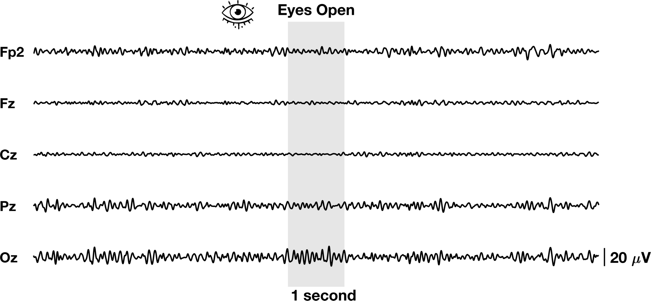
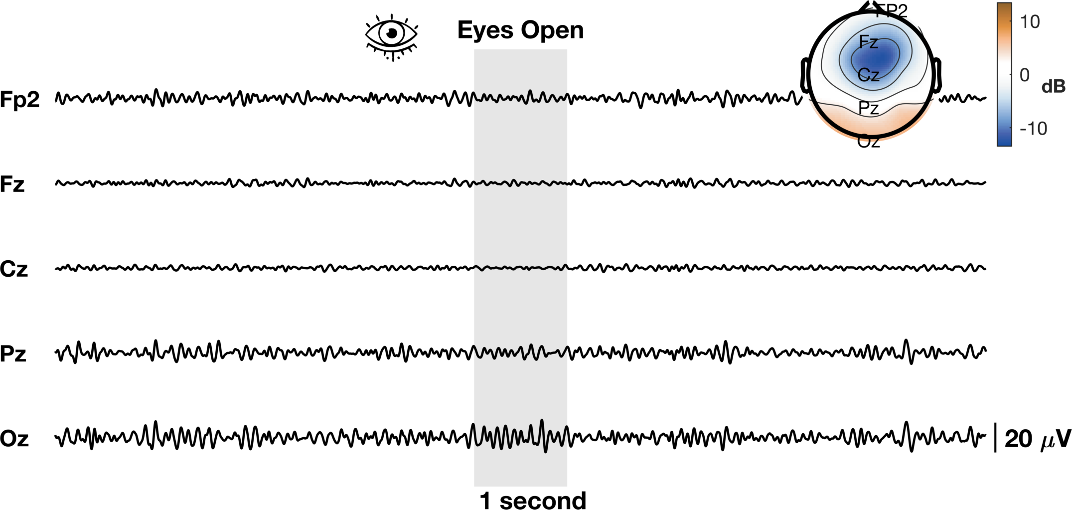
The process is almost identical to V2 with a few stylistic differences. In addition, we’ve added the grey bar instead of a line to show the 1 second window we plan to further highlight. Another way to visualize EEG data is to look at the distribution of band power in a specific time window across the entire scalp. We will use the topoplot.m function in eeglab. This function (along with many eeglab functions) can be finicky so we will need to do some hacky fixes to make it work like we want it to. It’s not perfect but it gets the point across.
%% Add topoplot to show alpha power
% Add topoplot
ax_topo  = axes('position',[0.675 0.7 0.275 0.275]);

% Get channel locations
[chanlocs, labels, Th, Rd, indices] = readlocs(fullfile(cd,'data','MotionTestChannelLocations_noEOG.ced'));

% %%%%%%%%%%%%%%%%%%%%%%%%%%%%%%%%%%%%%%%%%%%%%%%%%%%%%%%%%%%%%%%%%%%%%%%%
% %%%%%%%%%%%%%%%%%%% TOPOPLOT HACK %%%%%%%%%%%%%%%%%%%%%%%%%%%%%%%%%%%%%%
% %%%%%%%%%%%%%%%%%%%%%%%%%%%%%%%%%%%%%%%%%%%%%%%%%%%%%%%%%%%%%%%%%%%%%%%%

% This section is for updating the topoplot. This is a very hacky way of
% doing this, but for this example it will suffice. In order to update the
% topoplot in the loop, we either need to remake the topoplot every
% iteration (VERY BAD!) or go into the code and determine how the scalp map
% is being computed. That is what is happening below. Here, all the
% parameters required to compute the surface plot are being precomputed.
% Thus, only the surface plot will need to be updated each iteration and
% the new color data will be updated in the topoplot.

Th = pi/180*Th;
[x,y]     = pol2cart(Th,Rd);
plotrad = min(1.0,max(Rd)*1.02);            % default: just outside the outermost electrode location
plotrad = max(plotrad,0.5);                 % default: plot out to the 0.5 head boundary
% default_intrad = 1;     % indicator for (no) specified intrad
% intrad = min(1.0,max(Rd)*1.02);             % default: just outside the outermost electrode location
 rmax = 0.5;
% headrad = rmax;
% allx      = x;
% ally      = y;
squeezefac = rmax/plotrad;
intRd = Rd;
intTh = Th;
intx = x;
inty = y;
% intRd = intRd*squeezefac; % squeeze electrode arc_lengths towards the vertex
% Rd = Rd*squeezefac;       % squeeze electrode arc_lengths towards the vertex
%                           % to plot all inside the head cartoon
intx = intx*squeezefac;
inty = inty*squeezefac;
% x    = x*squeezefac;
% y    = y*squeezefac;
% allx    = allx*squeezefac;
% ally    = ally*squeezefac;
xi = linspace(-.5,0.5,67);   % x-axis description (row vector)
yi = linspace(-.5,0.5,67);
delta = xi(2)-xi(1); % length of grid entry

% %%%%%%%%%%%%%%%%%%%%%%%%%%%%%%%%%%%%%%%%%%%%%%%%%%%%%%%%%%%%%%%%%%%%%%%%
% %%%%%%%%%%%%%%%%%%%%%%%%%%%%%%%%%%%%%%%%%%%%%%%%%%%%%%%%%%%%%%%%%%%%%%%%


% Get alpha power limits
log_alpha = 10.*log10(all_alpha_power);
change_alpha = log_alpha - mean(log_alpha(:));
max_alpha = max(abs(change_alpha(:)));

% Compute alpha power in window
alpha_power_window = 10.*log10(sum(abs(all_alpha_data(:,round(midpoint-win_length/2):(round(midpoint-win_length/2)+win_length))).^2,2));
% Plot data using topoplot
tplot = topoplot(alpha_power_window- mean(log_alpha(:)),chanlocs,'electrodes','off','numcontour',4,'whitebk','on','headrad',0.5);
hold on;
% Add topoplot showing channels with time series
tplot2 = topoplot([],chanlocs(chans2plot),'style','blank','electrodes','labels','hcolor','none','whitebk','on');

% Change scale
cbar = colorbar;
cbar.Position(1)      = .925;
cbar.FontSize         = 9;
cbar.Label.String     = 'dB';
cbar.Label.Rotation   = 0;
cbar.Label.FontWeight = 'b';
%cbar.Limits = [-max_alpha max_alpha];
colorscale = flipud(lbmap(100,'BrownBlue'));
colormap(colorscale);

% Change figure color back to white
fig3.Color = 'w';
Now lets animate the damn thing!
%% Animate
% Define values for animation
win         = [1 10*fs];
update_rate = 1/10;
win_length  = 1*fs;
count       = 1
filename = 'eeg_raster_finalanimated_v3_3.gif'

% Create play toggle button
PlayButton = uicontrol('Parent',fig3,'Style','togglebutton','String','Play','Units','normalized','Position',[0.01 0.01 .1 .05],'Visible','on',...
    'BackgroundColor','w');
% Create close button
CloseButton = uicontrol('Parent',fig3,'Style','togglebutton','String','Close','Units','normalized','Position',[0.89 0.01 .1 .05],'Visible','on',...
    'BackgroundColor','w');
% Pause to render
pause(0.01);

% Begin loop
start_time = tic;
while win(end) < size(alpha_data,2)
    if PlayButton.Value == 1
        PlayButton.String = 'Pause';
        if toc(start_time) < update_rate
            % do nothing
        else
            for ii = 1: size(alpha_data,1)
                ax(ii).Children(end).YData = alpha_data(ii,win(1):win(2));
                ax(ii).Children(end-1).YData = alpha_highlight(ii,win(1):win(2));
            end
            % Uncomment if debugging eyes open/closed above:
            % peyes_open.YData = eyes_open(win(1):win(2));
            midpoint= round((win(1)+win(2))/2);
            % Compute alpha power in window
            alpha_power_window = 10.*log10(sum(abs(all_alpha_data(:,round(midpoint-win_length/2):(round(midpoint-win_length/2)+win_length))).^2,2));
            % Plot data using topoplot
            changeInAlpha =alpha_power_window- mean(log_alpha(:));
            % Compute updated grid
            [Xi,Yi,Zi] = griddata(inty,intx,double(changeInAlpha),yi',xi,'v4'); % interpolate data
            % Mask - EEGLAB stuff
            mask = (sqrt(Xi.^2 + Yi.^2) <= 0.5); % mask outside the plotting circle
            ii = find(mask == 0);
            Zi(ii)  = NaN;                         % mask non-plotting voxels with NaNs
            % UPDATE TOPOPLOT
            tplot.CData = Zi;
            % Get index of first point entering rectangle
            xIDX = round(midpoint + win_length/2);
            switch eyes_open(xIDX)
                % Change to eyes closed
                case 0
                    ax_open.Title.String     = 'Eyes Closed';
                    ax_imopen.Children.CData = I_closed;
                    % Change to eyes open
                case 1
                    ax_open.Title.String     = 'Eyes Open';
                    ax_imopen.Children.CData = I_open;
            end
            % Shift window
            win = win + fs*update_rate;
            % Pause to allow everything to render
            pause(0.001);
            % Update start time
            start_time = tic;
        end
    elseif PlayButton.Value == 0
        PlayButton.String = 'Play';
    end
    pause(0.001);
    % Check if close button pressed
    if CloseButton.Value == 1
       break;
    end
    pause(0.001);

    % Capture the plot as an image
    frame = getframe(fig3);
    im = frame2im(frame);
    [imind,cm] = rgb2ind(im,256);
    % Write to the GIF File
    if count == 1
        imwrite(imind,cm,filename,'gif', 'Loopcount',inf,'DelayTime',0.1);
    else
        imwrite(imind,cm,filename,'gif','WriteMode','append','DelayTime',0.1);
    end
    count = count + 1;
end
close(fig3);
Awesome! So the final product now has a ton of information and we have an animation for presentations. I know the quality is pretty low. This is a consequence of how it is being exported. Also, it is sped up quite a bit just for this example. You also cannot see my mouse, but I am using the buttons to play/pause and close the animation. I am sure we can find a way to do a better job and get a higher resolution image, but for now I am happy with this.
Next time…
Join me for the next post on time-frequency plots of EEG data.